( ESNUG 575 Item 2 ) ---------------------------------------------- [08/25/17]

Subject: MunEDA mocks both Solido HSMC and Cadence SSS for lame Monte Carlo
... blah blah blah blah blah (Solido's) HSMC vs. our (Cadence Virtuoso) Scaled-Sigma Sampling (SSS) blah blah blah...
- TeamADE Cadence (Cadence.com 08/18/2016)
From: [ Michael Pronath of MunEDA ]
Hi, John,
It seems like Cadence reopened Solido's old wounds with their TeamADE blog
post, and since DeepChip is the "Switzerland" of EDA tool discussion, I
thought I'd add some MunEDA comments on this topic.
---- ---- ---- ---- ---- ---- ----
1. Solido HSMC has Verifiability Problems
Cadence Team ADE wrote in their blog about Solido HSMC that "the response
surface model may indicate a wrong tail region for subsequent sampling,
causing significant inaccuracy."
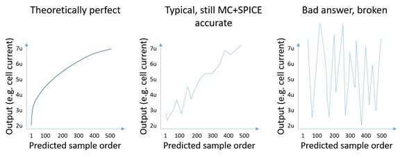
In ESNUG 562 #5 Solido's Jeff Dyck responds with this image:
and Jeff writes claiming:
"The middle graph shows a monotonically increasing plot with some
sorting noise - which is typical, and produces a perfect Monte Carlo
and SPICE accurate result. ... Solido HSMC automatically detects
ordering problems and reports them to the designer -- so it never
reports a bad answer. ... it's a 100% perfect match between what
brute force SPICE reports and what Solido HSMC reports. Zero
difference. ... Our HSMC also keeps the user informed of any such
issues and any corrections it did during runtime. No surprises."
But what Jeff wrote is all just wrong. What Solido doesn't want their users
to know: There may be a large error between the Solido HSMC results and the
true Monte Carlo analysis even if the sample plot is smooth and monotonic.
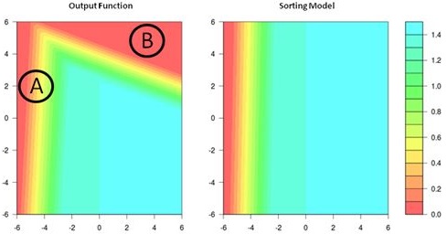
To show how easily this sample plot fails to detect severe ordering problems,
see this example output function and sorting model:
Fig.2: Output function in two variables with two connected failure
regions A and B. The model is a little inaccurate in region
A; the failures in region B are missing in the model.
This model misses a good part of failures and may cause ordering problems.
Solido doesn't tire of telling how 100% safe they think their HSMC is
because the magic sample plot can detect ordering problems. So let's
see how it works for this rather obvious case.
Let's generate 1 million standard normal random data points, sort them by
the model, and then evaluate the output function at the sorted sample.
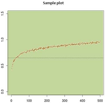
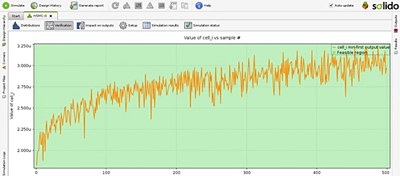
The sample plot of the simulation results of the first 500 data points (out
of 1M total) sorted by the model looks perfect:
Fig.3: Output function values plotted of the first 500 samples
that were sorted by the model. The dotted line marks
the lower spec limit 0.65.
The user doesn't know the output function nor the response surface model,
but only sees the sample plot of Fig.3. The model correlates well with
the true output function in these 500 samples. According to Solido's
logic we can stop simulation now because the very smooth sample plot
supposedly verifies a SPICE+MC accurate run.
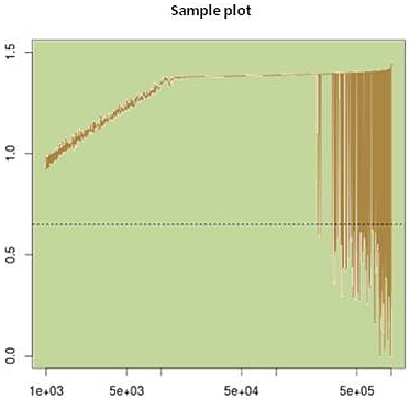
But if we don't fall for that and continue simulating the complete set of
1M sorted data points, then we'll eventually discover the truth and get
an ugly surprise when a lot of failures from region B show up late:
    Fig.4: Continued sample plot of Fig.3 from index 501 to 1,000,000
           (logarithmic x-axis).  Bad samples from region B were sorted
           wrongly by the model and don't show up until 200,000 more
           simulation runs -- which Solido misses!  The true MC failure
           rate is 248ppm (3.5 sigma) --- 10x larger than the estimate
           after the first 500 runs (24ppm, 4.1 sigma).

There is a fundamental difference between Solido HSMC and true Monte Carlo;
true MC simulates independent random samples distributed over the full
space.  True MC allows stopping anytime with calculating exact confidence
intervals on the results.

Whereas with Solido HSMC, a bad model may sort a lot of failures to the
end of the simulation queue, but nevertheless produce a falsely smooth
sample plot in the first few thousand simulation runs.  No matter when you
stop simulation and no matter how smooth the Solido plot is, one cannot give
confidence intervals nor say much about the error in HSMC results at all.

Solido HSMC users should ask themselves: How can they ever be sure when to
stop simulation if the Solido sample plot looks perfect but the majority
of failures may show up suddenly, millions of simulation runs later?

Solido HSMC verifiability is a false promise, as is "100% SPICE+MC accuracy."
Although the sample plot shows only simulated values, the model still has a
large influence on results such as failure rate or 6-sigma value.

A bad response surface model may cause a large undetectable error.

That's what Cadence correctly pointed out in its TeamADE blog -- but Solido
can't fix, Solido denies, and then Solido teaches their users to have blind
faith in black box models and truncated sample plots instead.

        ----    ----    ----    ----    ----    ----   ----

2. This is Really Just Sorting for a Global Minimization

Solido's Jeff Dyck shows this screenshot in ESNUG 562 #5:
and then Jeff writes claiming:
"By the time HSMC has run 500 samples, it has recovered the worst
case ~400 out of the population of 10 billion. This gives perfect
6 sigma Monte Carlo and SPICE accuracy in the worst case bit cell
current tail."
The Solido estimate for the 6-sigma worst-case bit cell current from this
plot is about 2.2uA (since in 10 billion samples, about 10 are worse than
the 6-sigma/1ppb quantile, and in this plot about 10 are worse than 2.2uA).
Estimating the 6-sigma worst-case bit cell current from these 500 samples
relies on the idea that the 10 worst sample points are here in these first
500 simulated samples. HSMC doesn't have to predict the currents of the
other 9,999,999,500 samples accurately, but it must be absolutely sure that
their true values are all larger than 2.2uA if simulated.
That means, the response surface model must be able to identify the true
global minimum of the "read" current in the sample cloud, in order to
really sort the worst samples to the front of the simulation queue. Else,
if sorting by the model identified only a local minimum of the true
values, then a malfunction like in Fig.4 will happen.
Jeff Dyck adds in ESNUG 562 #5:
"Sorting models are much easier to make (compared to response surface
models that predict precise output values.) A sorting model just
needs to figure out the order of samples in output space."
The Solido folk seem not to be aware that "just figure out the order of
samples" includes global minimization of the sample's true output function.
Global minimization of arbitrary output functions is much more difficult
than fitting a response surface model with some average error.
---- ---- ---- ---- ---- ---- ----
---- ---- ---- ---- ---- ---- ----
---- ---- ---- ---- ---- ---- ----
3. Cadence SSS is Averaging; while Solido HSMC is Black Box
The Cadence TeamADE guys wrote in their blog:
"Scaled-Sigma Sampling (SSS) generates a reasonably large number of
samples in the actual failure region without making assumptions.
These more predictive samples are then used to estimate the
failure rate."
The CDNS R&D folks first explained their Scaled Sigma Sampling (SSS)
method in detail in their 2013 ICAD paper
Shupeng Sun et al: "Fast Statistical Analysis of Rare Circuit
Failure Events via Scaled-Sigma Sampling for High-Dimensional
Variation Space." IEEE TCAD vol.37
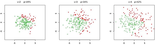
SSS works in three steps:
1. Run standard Monte Carlo but with a constant scaling factor "s"
on all random variables. Do this at least 3 times with different
scaling factors "s", for example s=2, s=3, s=4, and estimate
failure rates "p" from these MC runs.
Notice the three scaled MC runs in SSS with same sample size and
scaling factors 2, 3, and 4. A larger scaling factor "s" will
produce a larger portion "p" of failing samples (red).
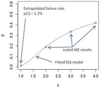
2. Fit the special SSS model
log(p) ~ a + b*log(s) + c/s^2
using the simulated failure rates and scaling factors by a least
squares fit for coefficients a, b, and c.
3. Extrapolate the model to
s=1: p=exp(a+c)
This is the final failure rate estimate.
    This graph is fitting the SSS model and extrapolating to s=1.

SSS is interesting because it can be performed with standard MC tools and
needs no model in the parameter space.  This sets it apart from adaptive
importance sampling, HSMC, or worst-case analysis.

The question is of course, how accurate is this model and what are its
limitations?

Let's see how it performs on a simple analytic example for which we know
the exact solution.
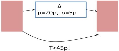
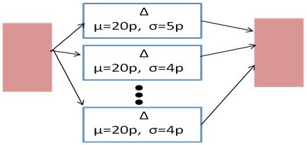
    Fig.5: One path with 20 psec mean delay and standard deviation
           5 psec.  No matter what, the delay must not exceed 45 psec.

Run scaled Monte Carlo, with 5 different scaling factors s = {2,3,4,5,6}
on this path.  For example, a scaling factor s=3 means we run Monte Carlo
with 3*5psec == 15 psec standard deviation on the delay element, and find
that 4.779% of samples exceed the limit 45 psec; hence p(s=3) = 0.04779.

                  scaling factor s     failure rate p
                        2.0                 0.00621
                        3.0                 0.04779
                        4.0                 0.10565
                        5.0                 0.15866
                        6.0                 0.20233

We fit the SSS model to this data, to get

                        a = -2.079, b = 0.477, c = -13.34

and evaluate the model at

                        s=1 : p == exp(a+c) == 2.017E-7

which is equivalent to 5.07 sigma of a normal distribution.

Thanks to using an analytical example we know the exact 5 sigma solution:

                   p == 1 - F((45-20)/5) == 1 - F(5) == 2.867E-7

where F(.) as the standard normal cumulative distribution function.

The SSS result is quite close to the exact value.  (Good!)

        ----    ----    ----    ----    ----    ----   ----

But how does the failure rate model perform if we add other, non-critical
failure modes?  Let's add some 10 more paths in parallel, but with 20%
less variation than this critical first one, so that they won't influence
the true result:
    Fig.6: Adding 10 more non-critical paths.  Again. the maximum delay
           must still not exceed 45 psec.

Using an analytical example, we know the exact 4.999 sigma failure rate:

                p == 1 - F((45-20)/5) * F((45-20)/4)^10 == 2.887E-7

Almost the same for the one critical path alone; these 10 additional non-
critical paths really don't make a difference.

But such non-critical failure modes distort the failure rate of scaled MC
runs a lot when we apply SSS:

                  scaling factor s     failure rate p
                        2.0                 0.01501
                        3.0                 0.21087
                        4.0                 0.51358
                        5.0                 0.72454
                        6.0                 0.84070

When we fit the SSS model to this new data, and evaluate the model at

                        s=1 : p == exp(a+c) == 4.152E-9

equivalent to 5.76 sigma of a normal distribution.

        ----    ----    ----    ----    ----    ----   ----

THIS IS WHERE CADENCE SSS FAILS

The end results are:

           Cadence SSS says 4.152E-9 vs. Solido HSMC says 2.887E-7

That's a major mistake where Cadence SSS underestimates the failure
rate by 70x!   Fig.6 is an example how Cadence SSS can fail.   2.887E-7 is
the correct result.

        ----    ----    ----    ----    ----    ----   ----

AND NOW WHERE SOLIDO HSMC ALSO FAILS

But also Solido HSMC can give bad results, too.  Why?  One can't say for
sure what the Solido result will be because their model is a black box.
After building a sorting response surface model for the maximum delay of
all paths, in the best case the Solido black box model identifies the
critical path and reports the correct failure rate.

In the worst case, the Solido sorting model overlooked the critical path
and models only one of the many non-critical paths just like in Fig.2.

If that happens then the result will be p=2.052E-10 (6.25 sigma) and
then Solido HSMC underestimates the failure rate by 1400x, but still shows
a misleadingly smooth and monotonic sample plot when simulating the
sorted samples.

        ----    ----    ----    ----    ----    ----   ----

While Cadence SSS does not create a model of the output function nor failure
region, the validity of the SSS failure rate model still depends on the
shape of the failure region.  Additional non-critical (seemingly irrelevant)
failure modes make the SSS estimate optimistic.

While Solido HSMC will have a large undetectable error when the model misses
the critical failure mode, SSS accuracy suffers from averaging over all
failure modes.

        ----    ----    ----    ----    ----    ----   ----

It starts to become apparent now: the whole point of high sigma analysis is
to identify the most probable (critical) failure mode -- a problem that's
equivalent to doing global optimization.

        ----    ----    ----    ----    ----    ----   ----

4. All High-Sigma Analysis is actually Global Minimization

High sigma simulation is easier to understand once we look at the difference
between low sigma and high sigma failure distribution densities.  See this
example of a failure region with strongly nonlinear bounds in the space of
mismatch parameters.  The graph on the right side shows the density of
Monte Carlo samples that fail:
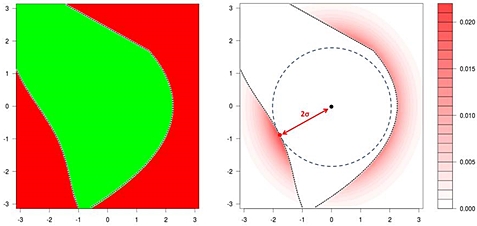
Fig.7: Monte Carlo simulation of a 2-sigma case in two standard
normal random variables, such as mismatch parameters of two
MOS. Left panel: region of failing samples (red) and region
of good samples (green). Right panel: probability density
of failing samples. Failing samples are distributed over
a large region.
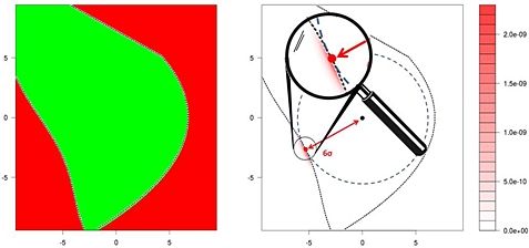
The density looks notably different for a high-sigma analysis case in Fig.8
below: (identical shape of failure region but consider the axes; it has a
3x higher robustness)
Fig.8: Monte Carlo simulation of a 6-sigma case. Failing samples
of a true Monte Carlo run are highly concentrated at the most
probable point (red halo at the red dot under a magnifying
glass). Other parts of the failure region, even if only 10%
further away, contribute to the failure rate only marginally.
Estimating failure rate in Fig.8 is a trivial local integration problem that
can be solved with little effort and high accuracy once we know the most
probably point (MPP, also known as worst-case point WCP). Knowing the WCP
in Fig.8 exactly allows estimating the failure rate with an error equivalent
to the sampling error of 1E12 MC runs, much more accurately than running
only 10E9 samples.
High-sigma analysis is better seen foremost as a global search problem, and
to a much lesser extent as an integration problem.
The WCP is the global maximum of the probability density in the failure
region. There may be multiple local maxima. Search methods for the WCP
can take measures to improve chances of finding the global maximum and not
just a local one. But the worst-case point is not only relevant for search
methods; it is just as important for Solido HSMC and Cadence SSS.
Sorting samples in a model like how Solido HSMC does is one way to find the
global maximum of the failure density in the model.
Cadence SSS estimates the low-sigma failure rate in Fig.7 and extrapolates
it to the high-sigma case of Fig.8 without knowing the location and distance
of the WCP. The curved right side of the failure region adds bias to the
SSS result because it is irrelevant at high sigma but strongly influences
the scaled MC runs.
When searching the worst-case point, local accuracy and convergence checks
make a big difference. EDA tools that estimate the failure rate from only
a rough guess of the worst-case point produce a large error. That's not a
reason to abandon the worst-case point, but rather to determine WCP more
accurately.
---- ---- ---- ---- ---- ---- ----
5. Practical Relevance & the Verifiability Problem
Is this local/global minimum issue relevant for typical high-sigma analysis
cases such as SRAM bit cell characterization, or delays in custom cells?
Yes, it is for some specs -- and every method (HSMC, DMIS, MPP/WCP search,
SSS, ...) may produce large errors without warning by missing the global
worst-case point. There is no "verifiability".
EDA tool vendors should keep users aware of that and help them with creating
test benches and metrics that isolate individual failure modes. Fortunately
it's not difficult for the SRAM bit cell, or delay analysis, so that a fast
and accurate and safe analysis is feasible.
For practical purposes the results of worst-case analysis, HSMC, importance
sampling, or SSS will be almost the same. The real differences between the
methods are runtime, accuracy, and scalability.
---- ---- ---- ---- ---- ---- ----
6. Solido vs. MunEDA Runtimes and Scalability beyond 5 Sigma
Regarding SSS, the failure rates of example cases that Cadence published
in IEEE TCAD vol.37 are still larger than 7.9E-7 and do not yet reach
5 sigma. The confidence interval they give for a sample size of 10k for
this case is [6.5E-9, 8.2E-6] or [4.3, 5.7] sigma. I don't know if this
will scale to 6 sigma and beyond with an accuracy of +-0.1 sigma and a
tolerable effort.
Regarding Solido HSMC, runtime will be an issue. When Amit Singhee and Rob
Rutenbar published the idea of simulating a subset of a huge sample picked
by a response surface model / classifier, at DATE 2007 in Nice, it reminded
me of an approach that MunEDA shortly tried for estimating fault coverage
of analog testing, but had to abandon because evaluating billions of data
points in a non-linear model was too much in the late 1990s and we would've
needed orders of magnitude more.
In ESNUG 562 #5 Jeff Dyck writes
"To measure cell current on a SRAM bit cell to 6-sigma, Solido HSMC
would: (...) This job would take 1500 simulations, about 2-3 minutes
of algorithmic runtime, and around 5 minutes of simulation time
using 15 SPICE simulators in parallel."
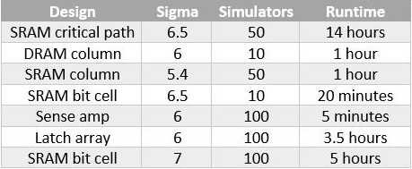
and Jeff shows this table of HSMC runtimes and effort:
Obviously the analysis effort for the SRAM bit cell grows dramatically with
# of samples run in the model, from 6 sigma to 6.5 sigma, and 7 sigma.
Who would've thought that generating 6 trillion random data vectors and
evaluating them all in a response surface model is a quite inefficient
global minimization method -- particularly for rather well known SRAM
bit cell metrics? :)
The effort to solve a high sigma analysis case need not depend on the
sigma level. A good high sigma analysis tool can run a 7-sigma analysis
of an SRAM bit cell just as fast as for 6-sigma or 5-sigma. Efficiency
matters. For many practical applications, high-sigma analysis is run in
sweeps over corners, design options, voltage levels,... possibly
hundreds of times.
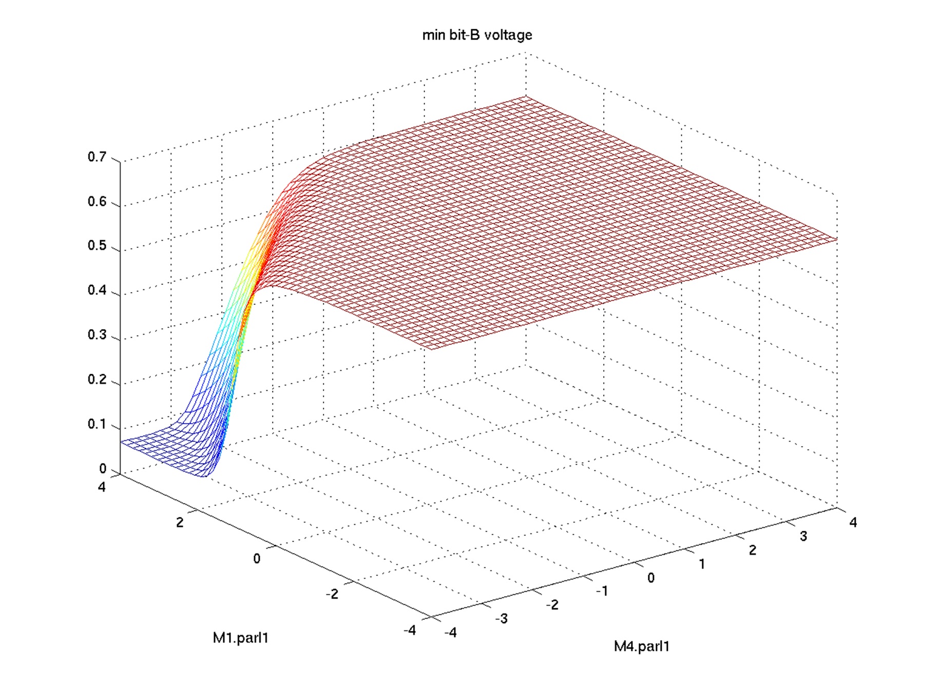
Hongzhou Liu of Cadence showed in ESNUG 523 #08 how voltage output levels
of a bit cell depend on mismatch variables:
Fig 9. Hongzhou's bit voltage vs statistical variables plot
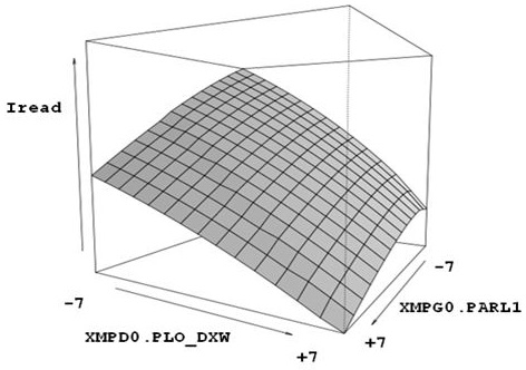
and this is how the "read" current of a 28nm SRAM bit cell depends on two
sensitive parameters:
Finding the global minimum of this function within a 7-sigma distance to the
center shouldn't be too hard. MunEDA WiCkeD needs about 90 secs on 1 host
machine -- including all SPICE runs -- for that. Whoever spends 5 hours on
100 hosts to evaluate a trillion points in this plot can certainly find a
better use of his time. :)
---- ---- ---- ---- ---- ---- ----
7. How MunEDA WiCked Trounces Solido HSMC
But rather than make this an empty claim against, Solido HSMC (which I know
you hate EDA vendors doing, John), here's the detailed step-by-step way
MunEDA WiCkeD does it.
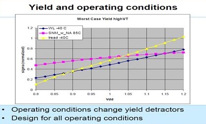
1) These are (normalized) 6-sigma worst-case sweeps of SRAM bit
cell specs with MunEDA WiCkeD, that show how the dominant
yield detractor depends on Vdd.
Fig.9: The relative importance of the failure modes, as
well as the relative importance of individual
devices' variation, depends on temperature, Vdd,
global process corners, aging, design options, ...
Repeating high-sigma analysis in sweeps is a
must-have.
Our WiCkeD users have run high-sigma analysis in such sweeps for
SRAM characterization productively for the past 15 years. These
extensive high-sigma analysis runs are also helpful for yield
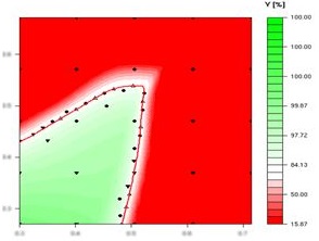
analysis and adjusting the process (yield ramp up):
Fig.10: Simulated array yield plot of a 28nm 16 MBit SRAM
array for multiple bit cell specs combined, plotted
over two process control measurements (PCM) on
the x- and y-axis.
These plots help to identify the process window with high SRAM
yield. About 40 high-sigma mismatch analysis runs are needed for
one plot including iterative refinement of a user-defined array
yield contour level.
Total runtime for one plot is about 2 hours on 2 simulation hosts.
MunEDA WiCkeD can generate such plots for various combinations of
Vdd and temperature, with some 600 high-sigma analysis runs total.
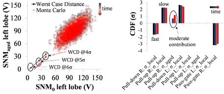
2) A worst-case distances (WCD) methodology can include aging. The
BTI effect in smaller nodes is a random process that adds variation
(aging induced dispersion). STMicroelectronics included the
effect when analyzing FDSOI bit cells (published at IRPS 2016):
Fig.11: Worst-case values and worst-case sensitivities
depend on aging stress over time.
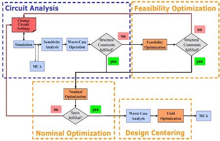
3) The holy grail of variation aware design is circuit optimization.
That is, coupling high sigma analysis with a multi-objective
constraint-based optimization tool to optimize the tradeoffs
between robustness, reliability, area, performance, and power.
You need a high sigma analysis method that is not only accurate
and fast, but that can also provide sensitivities of spec
robustness with respect to device geometries.
Here's the MunEDA cell optimization flow that we use for sense
amps, bandgaps, I/O, and bit cells:
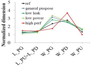
In this way WiCkeD can generate cells for different purposes:
These are the MunEDA WiCked results of sizing bit cells for different
performance requirements.  Geometry variables on the x-axis, optimization
results on the y-axis.  Optimization is performed to fulfill nominal
performances (standby current, read current) and WCD criteria for SNM
and WM using a footprint constraint.

You can do a reliable MunEDA high sigma run in minutes with a transparent
method and easy plausibility checks; or a Solido HSMC run in days with a
black box model and the illusion of verifiability; or a Cadence SSS run
with a potentially large bias and no plausibility checks.  Your choice.

    - Michael Pronath
      MunEDA GmbH                                Munich, Germany

        ----    ----    ----    ----    ----    ----   ----

|
Michael Pronath has been doing REALLY complicated EDA tool dev for 19 years. He has a PhD and he's German. They don't make mistakes. They're not allowed to.
|
Related Articles:

    Solido's new brainiac, Jeff Dyck, calls out CDNS HSMC attack blog
    BDA, Solido, MunEDA, and Silvaco get #5 for Best EDA of 2016
    Solido brainiac Trent on user comments, and MunEDA WCD questions
    Virtuoso R&D and LibTech still both doubt Solido's 6-sigma claims
    263 engineers on their present day SPICE use and SPICE leaders
Join
Index
Next->Item
|
|